Pandas: Reproduction of Microarray Study Results
This is a step-by-step guide to reproduce the results of a microarray study by using Pandas, scikit-learn, and other Python scientific libraries. Here, my target is the principal component analysis (PCA) conducted in Lukk M, Kapushesky M, Nikkilä J, et al. A global map of human gene expression. Nat Biotechnol. 2010;28:322-324. doi:10.1038/nbt0410-322.
Data retrieval
The authors provide all their datasets at the repository 'E-MTAB-62 - Human gene expression atlas of 5372 samples representing 369 different cell and tissue types, disease states and cell lines.' Let's look and see what's there.
Four files are listed in addition to lots of raw data. Namely,
- E-MTAB-62.idf.txt
- Investigation description
- E-MTAB-62.sdrf.txt
- Sample and data relationship
- E-MTAB-62.processed.2.zip
- Microarray data processed, tab-seperated, and compressed
- A-AFFY-33.adf.txt
- Array design
First, I import Python modules I need in this project.
import pandas as pd
import seaborn as sns
from matplotlib import pyplot as plt
from sklearn.decomposition import PCA
Next, I load E-MTAB-62.sdrf.txt to associate sample attributes such as cell types and origins with the microarray data to be downloaded soon.
sample_data_rel = pd.read_csv(
    'https://www.ebi.ac.uk/arrayexpress/files/E-MTAB-62/E-MTAB-62.sdrf.txt',
    sep='\t',
    index_col='Source Name'
)
sample_data_rel consists of 33 columns for sample attributes and 5372 rows for as many samples. For example, the column "Characteristics[4 meta-groups]" indicates that a sample is related to which of neoplasm, cell line, normal, and disease.
>>> sample_data_rel['Characteristics[4 meta-groups]'].value_counts()

neoplasm     2315
cell line    1256
normal       1033
disease       765
Name: Characteristics[4 meta-groups], dtype: int64
Most samples derive from humans, but surprisingly, there happen to be a few mouse samples as well.
>>> sample_data_rel['Characteristics[Organism]'].value_counts()

Homo sapiens    5369
Mus musculus       3
Name: Characteristics[Organism], dtype: int64
I get rid of them since I need only human data.
sample_data_rel = sample_data_rel.loc[
    sample_data_rel['Characteristics[Organism]'] == 'Homo sapiens'
]
Below is the complete list of sample attributes and variables.
Then I load E-MTAB-62.processed.2.zip, the processed microarray data.
affymetrix = (
    pd.read_csv(
        'https://www.ebi.ac.uk/arrayexpress/files/E-MTAB-62/E-MTAB-62.processed.2.zip',
        sep='\t',
        index_col='Hybridization REF',
        dtype='object' #1,2
    )
    .drop('CompositeElement REF') #3
    .astype('float32') #4
    .T #5
    .loc[sample_data_rel.index] #6
)
- The string 'RMA' in the 2nd row "CompositeElement REF" prevents conversion to floating point values and triggers an annoyingly long warning unless dtype is specified as 'object.' Skipping the row by adding a parameter
skiprows=[1]won't help avoid the bother. - The data occupy 8.1 GB of memory at this point.
- The 2nd row gets removed.
- By converting the values to float32, the data size is now reduced to 457 MB. Generally, three significant figures are more than sufficient in biology, and so float16 will be probably OK as well.
- The data consists of 22283 rows for as many genes and 5322 columns for as many samples. I transpose the matrix so that it is suitable for PCA, with samples in rows and genes in columns.
- I align the indices of this dataframe and sample_data_rel for convenience and also to remove the mouse portion of the data.
The microarray data is standardized sample-wise, as is stated in the paper's supplementary material and evidenced by the low variances in data distribution across samples (below).
>>> descr = (
    affymetrix
    .T # transposed back to the original format
    .describe()
)

>>> pd.merge(
    descr.mean(axis=1).rename('mean'),
    descr.var(axis=1).rename('variance'),
    left_index=True,
    right_index=True
)

        mean       variance
count   22283.00   0.000000
mean    6.876087   0.016922
std     1.795443   0.004527
min     3.461061   0.001730
25%     5.563369   0.005386
50%     6.723452   0.001895
75%     7.967647   0.007483
max     14.25868   0.024582
PCA
Finally, I get scikit-learn to perform PCA...
n_components = 2
pca = PCA(n_components=n_components)
Xp = pca.fit_transform(affymetrix)
Xp = pd.DataFrame(
    Xp,
    index=affrymetrix.index,
    columns=[f'PC{k+1}' for k in range(n_components)]
)
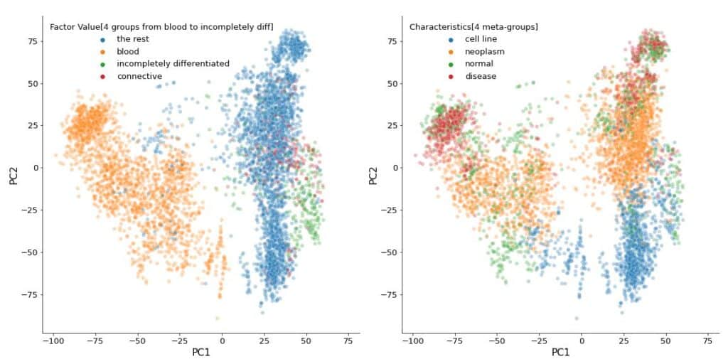
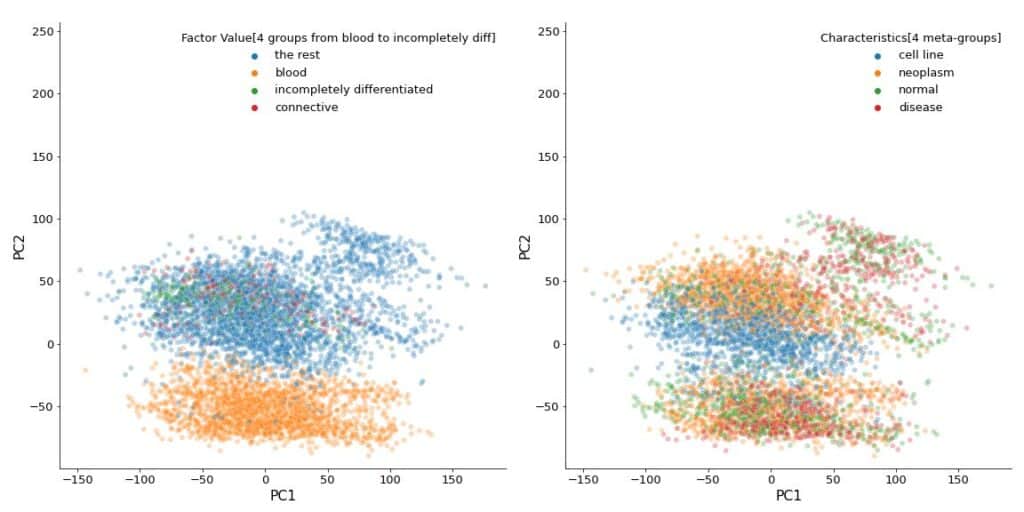
... and plot the results.
fig, axes = plt.subplots(nrows=1, ncols=2, figsize=(20, 10))
for i, col in enumerate(
    [
        'Factor Value[4 groups from blood to incompletely diff]',
        'Characteristics[4 meta-groups]'
    ]
):

    sns.scatterplot(
        ax=axes[i],
        data=Xp,
        x='PC1',
        y='PC2',
        hue=sample_data_rel[col],
        alpha=0.3,
    )
    axes[i].axis('square')

These plots appear identical to those in the paper.
If, as usual, I normalized the dataset, which is already normalized sample-wise as I wrote above, it would be doubly normalized (sample-wise and gene-wise) and give totally different results.
from sklearn.preprocessing import StandardScaler

sc = StandardScaler()
X = sc.fit_transform(affymetrix)
Xp = pca.fit_transform(X)
Xp = pd.DataFrame(
    Xp, index=affymetrix.index, columns=[f'PC{k+1}' for k in range(n_components)]
)

fig, axes = plt.subplots(nrows=1, ncols=2, figsize=(20, 10))
for i, col in enumerate(
    [
        'Factor Value[4 groups from blood to incompletely diff]',
        'Characteristics[4 meta-groups]'
    ]
):

    sns.scatterplot(
        ax=axes[i],
        data=Xp,
        x='PC1',
        y='PC2',
        hue=sample_data_rel[col],
        alpha=0.3,
    )
    axes[i].axis('square')


