Stacked Bar Chart in Python - Advanced

2024-06-27 2024-06-27

Hide

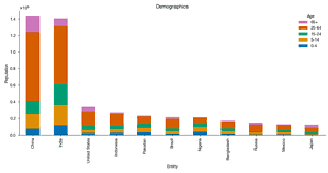
In this advanced tutorial, we delve deeper into the art of creating stacked bar charts using Python. Building upon our previous basic tutorial, we explore more sophisticated techniques to handle complex data structures and add attributes to our visualizations. We utilize data from Our World in Data to craft a country and age demographic stacked bar chart, and then we take on a new challenge: visualizing sales data for car models by different manufacturers.

We begin by installing necessary external libraries and importing data from goodcarbadcar.net into a Pandas dataframe. The tutorial guides you through the process of creating a ranking of year-to-date sales by brand and setting up the aesthetics for our graph. Instead of relying on Pandas’ plot.bar method, we employ Matplotlib’s features to meticulously stack bars and use the bar_label method to annotate models with significant sales.

Getting Started

Make sure you have the necessary libraries installed. Use conda install requests pandas matplotlib seaborn -y or pip install requests pandas matplotlib seaborn -y.

Data Preparation

Importing Data: Read the sales data into a Pandas dataframe. Split the ‘Model’ column into separate ‘Brand’ and ‘Model’ columns for better analysis.

import io
import re
import requests

url = 'https://www.goodcarbadcar.net/2023-us-vehicle-sales-figures-by-model/'
content = requests.get(url).content
tables = pd.read_html(io.StringIO(content.decode('utf-8')))
sales = (tables[0]
         .assign(Brand=lambda df: df.Model.str.split(n=1, expand=True)[0],
                 Model=lambda df: df.Model.str.split(n=1, expand=True)[1]
                 .replace('3', 'Mazda 3'))
         [['Brand', 'Model', 'YTD']]
         .dropna()
         .astype({'YTD': 'int'})
         )
sales.head()

Brand	Model	YTD
Mazda	Mazda 3	15157
Toyota	4Runner	57020
Volvo	60-Series	8788
Volvo	90-Series	697
Honda	Accord	68124

If the above link doesn't work, load the local data instead.

url = 'https://abittechnical.work/wp-content/uploads/2024/06/vehicle_sales.csv'
content = requests.get(url).content
sales = pd.read_csv(io.StringIO(content.decode('utf-8')))

Sales Ranking: Calculate the year-to-date (YTD) sales by brand. Group the data by brand and sum the sales.

ranking_by_brand = (sales
                    .groupby('Brand')
                    .YTD
                    .sum()
                    .sort_values(ascending=False)
                    )

Customizing the Chart

Matplotlib Aesthetics: Customize the appearance of the chart using Matplotlib. Adjust colors, fonts, and other visual elements to make the chart informative and visually appealing.

from matplotlib import pyplot as plt
from matplotlib import rcParams

rcParams.update(
    {
        "axes.spines.top": False,
        "axes.spines.right": False,
        "axes.formatter.use_mathtext": True,
        "axes.formatter.limits": [-3, 3],
        "lines.linewidth": 1,
        "legend.frameon": False,
        "font.size": 11,
        "text.usetex": False,
        "font.family": ["Helvetica Neue", 'DejaVu Sans', "IPAexGothic", "sans-serif"],
        'svg.fonttype': 'none',
    }
)

Stacking Bars Manually: Instead of relying on Pandas’ plot.bar method, manually stack the bars using Matplotlib. This gives you more control over the chart’s layout. Use the bar_label method to annotate models with significant sales over 30,000 units.

import numpy as np
import pandas as pd
import seaborn as sns
from cycler import cycler

n = 10
threshold = 30_000
width = 0.5
rcParams.update({'axes.prop_cycle': cycler(color=sns.color_palette('bright'))})
fig, ax = plt.subplots(figsize=(12, 6.3))

for i in range(n):
    brand = ranking_by_brand.index[i]
    df = (sales[sales.Brand == brand]
          .sort_values('YTD', ascending=False)
          .set_index('Model')
          [['YTD']]
          )

    bottom = np.zeros(1)
    for model, model_sales in df.iterrows():
        p = ax.bar([brand],
                   model_sales,
                   width=width,
                   bottom=bottom,
                   alpha=.4
                   )
        bottom += model_sales
        if model_sales.values[0] > threshold:
            name = model
        else:
            name = ''
        ax.bar_label(p, labels=[name], label_type='center')
ax.set_xlabel('Brand')
ax.set_ylabel('Sales volume')
ax.set_title(f'U.S. Vehicle Sales Volumes Ranking: Top {n}')
plt.tight_layout()

Conclusion

By following these steps, you’ll create advanced stacked bar charts that convey complex data effectively. Whether you’re a data scientist or a curious learner, mastering this technique will enhance your data visualization skills. Feel free to explore this tutorial and adapt it to your specific data sets.