Data-Driven Science and Engineering. Chapter 3 Exercises
I used Python and worked on exercises in Chapter 3 of Data-Driven Science and Engineering, 2nd Edition (2022).
Preliminaries
%matplotlib inline
import io
from pathlib import Path
import urllib
import pandas as pd
import numpy as np
import scipy
from matplotlib import rcParams
from matplotlib import pyplot as plt
from matplotlib.image import imread

A4 = [8.27, 11.69]

rcParams.update(
    {
        "axes.spines.top": False,
        "axes.spines.right": False,
        "axes.formatter.use_mathtext": True,
        "axes.formatter.limits": [-3, 3],
        "lines.linewidth": 1,
        "lines.markersize": 5,
        "lines.markeredgewidth": 0.5,
        "lines.markeredgecolor": "white",
        "legend.frameon": False,
        "font.size": 11,
        "text.usetex": False,
        "font.family": ["Helvetica Neue", "IPAexGothic", "DejaVu Sans", "sans-serif"],
        "axes.prop_cycle": plt.cycler("color", sns.color_palette("colorblind")),
    }
)

def download(url):
    obj = io.BytesIO()
    user_agent = "Mozilla/5.0 (Windows NT 6.1; Win64; x64)"
    headers = {"User-Agent": user_agent}
    req = urllib.request.Request(url, None, headers)
    with urllib.request.urlopen(req) as response:
        obj.write(response.read())
    return obj

def normalize(a):
    return a / (a.max() - a.min())

url_dog = "https://abittechnical.work/wp-content/uploads/2023/08/dog.jpg"
dogpict_original = imread(download(url_dog), format="jpg")
Exercise 3.1
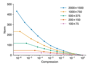
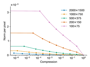
Load the image dog.jpg and convert to gray scale. We will repeat Exercise2.1, using the FFT to compress the image at different compression ratios. However, now, we will compare the error versus compression ratio for the image downsampled at different resolutions. Compare the original image (2000 × 1500) and downsampled copies of the following resolutions: 1000 × 750, 500 × 375, 200 × 150, and 100 × 75. Plot the error versus compression ratio for each image resolution on the same plot. Explain the observed trends.
steps = [1, 2, 4, 10, 20]
keeps = np.logspace(0, -6, 11)

fig, axes = plt.subplots(1, 2, figsize=(9, 3.6))
for step in steps:
    B = normalize(dogpict_original.mean(axis=-1)[::step, ::step])
    Bt = np.fft.fft2(B)
    Btsort = np.sort(np.ravel(np.abs(Bt)))
    h, w = B.shape
    norms = np.array([])
    label = str(h) + r"$\times$" + str(w)
    kept = []
    prev_ithreshold = np.inf
    for keep in keeps:
        ithreshold = int(np.floor((1 - keep) * len(Btsort)))
        if ithreshold == prev_ithreshold:
            continue
        prev_ithreshold = ithreshold
        threshold = Btsort[ithreshold]
        Atlow = Bt * (np.abs(Bt) > threshold)
        img = np.fft.ifft2(Atlow).real
        kept.append((np.abs(Bt) > threshold).sum() / (h * w))
        norms = np.concatenate([norms, [np.linalg.norm(B - img)]])
    axes[0].plot(kept, norms, "-o", label=label)
    axes[1].plot(kept, norms / (h * w), "-o", label=label)
for ax in axes:
    ax.legend()
    ax.set_xscale("log")
    ax.set_ylim(0, ax.get_ylim()[1])
    ax.set_xlabel("Compression")
axes[0].set_ylabel("Norm")
axes[1].set_ylabel("Norm per pixel")
Exercise 3.2
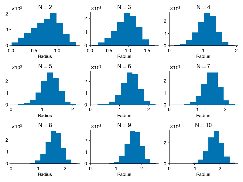
This example will explore geometry and sampling probabilities in high-dimensional spaces. Consider a two-dimensional square dart board with length L = 2 on both sides and a circle of radius R = 1 in the middle. Write a program to throw 10,000 darts by generating a uniform random x and y position on the square. Compute the radius for each point and compute what fraction land inside the circle (i.e., how many have radius < 1). Is this consistent with your expectation based on the area of the circle and the square? Repeat this experiment, throwing 10,000 darts randomly (sampled from a uniform distribution) on an N-dimensional cube (length L = 2) with an N-dimensional sphere inside (radius R = 1), for N = 2 through N = 10. For a given N, what fraction of the points land inside the sphere. Plot this fraction versus N. Also compute the histogram of the radii of the randomly sampled points for each N and plot these. What trends do you notice in the data?
M = 10000
Fraction = []
Ns = range(2, 11)
Radii = []
for N in Ns:
    darts = 2 * np.random.random([M, N]) - 1
    radii = np.linalg.norm(darts, axis=1)
    Radii.append(radii)
    fraction = (radii <= 1).sum() / M
    Fraction.append(fraction)

fig, ax = plt.subplots()
ax.plot(Ns, Fraction)
ax.set_ylim(ax.get_ylim() * np.array([0, 1]))
ax.set_xlabel("Dimension")
ax.set_ylabel("Fraction")
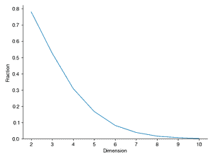
fig = plt.figure(figsize=(8, 6))
for i, N in enumerate(Ns):
    radii = Radii[i]
    ax = fig.add_subplot(3, 3, i + 1)
    ax.hist(radii)
    ax.set_title("N$=$" + str(N))
    ax.set_xlim(ax.get_xlim() * np.array([0, 1]))
    ax.set_xlabel("Radius")
plt.tight_layout()
Exercise 3.3
This exercise will explore the relationship between the sparsity \(K\), the signal size \(n\), and the number of samples \(p\) in compressed sensing.
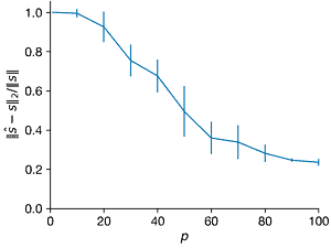
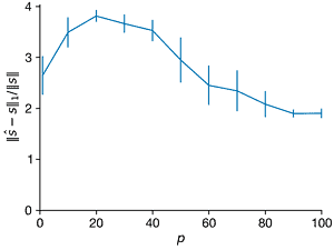
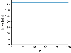
- For \(n = 1000\) and \(K = 5\), create a \(K\)-sparse vector s of Fourier coefficients in a Fourier basis \(\Psi\). For each \(p\) from 1 to 100, create a Gaussian random sampling matrix \(C ∈ R^{p×n}\) to create a measurement vector \(y = C \Psi s\). Use compressed sensing based on this measurement to estimate \(\hat{s}\). For each \(p\), repeat this with at least 10 realizations of the random measurement matrix \(C\). Plot the average relative error of \(||\hat{s} − s||_2/||s||\) versus \(p\); it may be helpful to visualize the errors with a box-and-whisker plot. Explain the trends. Also plot the average \(l_1\) and \(l_0\) error versus \(p\).
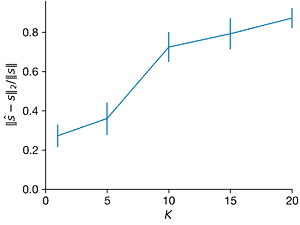
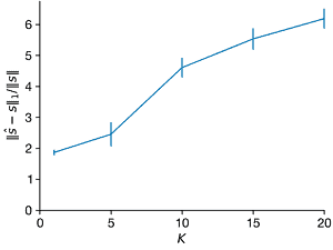
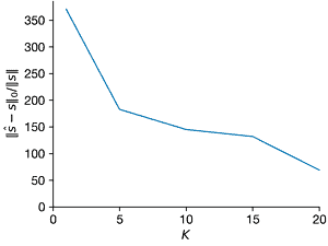
- Repeat the above experiment for \(K = 1\) through \(K = 20\). What changes?
- Now repeat the above experiment for \(K = 5\), varying the signal size using \(n = 100\), \(n = 500\), \(n = 1000\), \(n = 2000\), and \(n = 5000\).
L0_norm = lambda x: np.linalg.norm(x, ord=0)
L1_norm = lambda x: np.linalg.norm(x, ord=1)


def optimize_s(Theta, y):
    constr = {"type": "eq", "fun": lambda x: Theta @ x - y}
    x0 = np.linalg.pinv(Theta) @ y
    res = scipy.optimize.minimize(L1_norm, x0, method="SLSQP", constraints=constr)
    shat = res.x
    return shat


def estimate_s(p):
    C = np.identity(n)[np.random.permutation(n)[:p]]
    Theta = C @ Psi
    y = Theta @ s
    return optimize_s(Theta, y)

import pandas as pd

n = 1000
K = 5
repetition = 10
s = np.hstack([np.zeros(n - K), 5 * np.random.random(K)])[np.random.permutation(n)]
Psi = scipy.fftpack.dct(np.identity(n))

df1 = dict()
Ps = [1] + list(range(10, 101, 10))
for p in Ps:
    df1[p] = np.zeros([len(s), repetition])
    for i in range(repetition):
        shat = estimate_s(p)
        df1[p][:, i] = shat
df1 = pd.concat(
    {key: pd.DataFrame(val) for key, val in df1.items()},
        axis=1, names=["p", "round"]
)

norms1_l0, norms1_l0_sd = [], []
norms1_l1, norms1_l1_sd = [], []
norms1_l2, norms1_l2_sd = [], []

diff1 = df1 - np.tile(s, [len(Ps) * repetition, 1]).T
for p in Ps:
    norm0 = np.linalg.norm(
        diff1.loc[:, (p, slice(None))], ord=0, axis=0
    ) / np.linalg.norm(s)
    norm1 = np.linalg.norm(
        diff1.loc[:, (p, slice(None))], ord=1, axis=0
    ) / np.linalg.norm(s)
    norm2 = np.linalg.norm(
        diff1.loc[:, (p, slice(None))], ord=2, axis=0
    ) / np.linalg.norm(s)
    norms1_l0.append(norm0.mean())
    norms1_l0_sd.append(norm0.std(ddof=1))
    norms1_l1.append(norm1.mean())
    norms1_l1_sd.append(norm1.std(ddof=1))
    norms1_l2.append(norm2.mean())
    norms1_l2_sd.append(norm2.std(ddof=1))
fig, axes =  plt.subplots(1,3)
ax=axes[0]
ax.errorbar(Ps, norms1_l2, norms1_l2_sd, clip_on=False)
ax.set_xlim(0, max(Ps))
ax.set_ylim(ax.get_ylim() * np.array([0, 1]))
ax.set_xlabel("$p$")
ax.set_ylabel("$||\hat{s} - s||_2/||s||$")

ax=axes[1]
ax.errorbar(Ps, norms1_l1, norms1_l1_sd, clip_on=False)
ax.set_xlim(0, max(Ps))
ax.set_ylim(ax.get_ylim() * np.array([0, 1]))
ax.set_xlabel("$p$")
ax.set_ylabel("$||\hat{s} - s||_1/||s||$")

ax=axes[2]
ax.errorbar(Ps, norms1_l0, norms1_l0_sd, clip_on=False)
ax.set_xlim(0, max(Ps))
ax.set_ylim(ax.get_ylim() * np.array([0, 1]))
ax.set_xlabel("$p$")
ax.set_ylabel("$||\hat{s} − s||_0/||s||$")
Ks = [1, 5, 10, 15, 20]
p = 60

norms2_l0, norms2_l0_sd = [], []
norms2_l1, norms2_l1_sd = [], []
norms2_l2, norms2_l2_sd = [], []

sdict = dict()
df2 = dict()
for K in Ks:
    s = np.hstack([np.zeros(n - K), 5 * np.random.random(K)])[np.random.permutation(n)]
    sdict[K] = s
    diff = df2.loc[:, (K, slice(None))] - s.repeat(repetition).reshape(-1, repetition)
    df2[K] = np.zeros([len(s), repetition])
    for i in range(repetition):
        shat = estimate_s(p)
        df2[K][:, i] = shat
df2 = pd.concat(
    {key: pd.DataFrame(val) for key, val in df2.items()}, axis=1, names=["K", "round"]
)

norms2_l0, norms2_l0_sd = [], []
norms2_l1, norms2_l1_sd = [], []
norms2_l2, norms2_l2_sd = [], []

for K in Ks:
    s = sdict[K]
    norm0 = np.linalg.norm(diff, ord=0, axis=0) / np.linalg.norm(s)
    norm1 = np.linalg.norm(diff, ord=1, axis=0) / np.linalg.norm(s)
    norm2 = np.linalg.norm(diff, axis=0) / np.linalg.norm(s)
    norms2_l0.append(norm0.mean())
    norms2_l0_sd.append(norm0.std(ddof=1))
    norms2_l1.append(norm1.mean())
    norms2_l1_sd.append(norm1.std(ddof=1))
    norms2_l2.append(norm2.mean())
    norms2_l2_sd.append(norm2.std(ddof=1))
fig, axes = plt.subplots(1,3)
ax = axes[0]
ax.errorbar(Ks, norms2_l2, norms2_l2_sd, clip_on=False)
ax.set_xlim(0, max(Ks))
ax.set_ylim(ax.get_ylim() * np.array([0, 1]))
ax.set_xticks(range(0, 21, 5))
ax.set_xlabel("$K$")
ax.set_ylabel("$||\hat{s} − s||_2/||s||$")

ax = axes[1]
ax.errorbar(Ks, norms2_l1, norms2_l1_sd, clip_on=False)
ax.set_xlim(0, max(Ks))
ax.set_ylim(ax.get_ylim() * np.array([0, 1]))
ax.set_xlabel("$K$")
ax.set_ylabel("$||\hat{s} − s||_1/||s||$")

ax = axes[2]
ax.errorbar(Ks, norms2_l0, norms2_l0_sd, clip_on=False)
ax.set_xlim(0, max(Ks))
ax.set_ylim(ax.get_ylim() * np.array([0, 1]))
ax.set_xlabel("$K$")
ax.set_ylabel("$||\hat{s} − s||_0/||s||$")
